Beautiful lake tableaux to sketch

When I have done this exercise with college students, I’ve used that college’s racial demographic data, published by the Office of Institutional Research. This dataset leads to questions of categorisation (do they let students select multiple races, or do they simply select ‘multiracial’? Why are international students categorised separately?), which made their way into my students’ work.

Example – A Story That Examines a Trend

The example in this article walks you through building a story about earthquake trends over time.

The story feature in Tableau is a great way to showcase this type of analysis because it has a step-by-step format which lets you move your audience through time.

Rather than showing you how to create all the views and dashboards from scratch, this example starts from an existing workbook. What you’ll do is pull the story together. To follow along and access the pre-built views and dashboards, download the following workbook from Tableau Public: An Earthquake Trend Story (Link opens in a new window) .

Frame the story

A successful story is well-framed, meaning its purpose is clear. In this example, the story’s purpose is to answer the following question: Are big earthquakes becoming more common?

There are several approaches you could take—see Best Practices for Telling Great Stories for a list—but the one used here as an overall approach is Change over Time, because it works especially well for answering questions about trends. As you build the story you’ll notice that other data story types, such as Drill Down and Outliers, are blended in to support the overall approach.

Build the story

Create a story worksheet

1. Use Tableau Desktop to open the Earthquake Trend Story workbook that you downloaded. If you also have Tableau Server or Tableau Cloud and you want to do your authoring on the web instead of in Tableau Desktop, publish the workbook to your Tableau server, click Workbooks , select the workbook, then under Actions choose Edit Workbook . Once you open the workbook, you’ll see that it has three dashboards. You’ll be using those dashboards to build your story. The workbook also has a finished version of the story. Tip: To see the individual views that are in a dashboard, right-click the dashboard’s tab and select Unhide all Sheets .
2. Click the New Story tab. Tableau opens a new worksheet as your starting point.
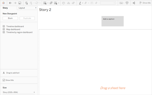
3. Right-click the Story 2 tab, choose Rename Sheet , and type Earthquake story as the worksheet name.

State the question

Story titles are in view at all times and they’re a handy way to keep your story’s purpose front and center. By default, Tableau uses the worksheet name as the story title. In Tableau Desktop you can override that by doing the following:

1. Double-click the title.
2. In the Edit Title dialog box, replace with the following: Are big earthquakes on the rise?
3. Click OK . If you’re authoring in Tableau Server or Tableau Cloud, the story tab is the only place where you can change the title.

Start big

To help orient your audience, the first story point you create will show the broadest possible viewpoint—all earthquakes, across the entire planet.

1. On the Story pane, double-click Map dashboard to place it on the story sheet. If you’re using Tableau Desktop, you can also use drag-and-drop to add views and dashboards to a story sheet. Notice how there’s a horizontal scroll bar and the legend isn’t fully displayed. There’s a special setting you can use on your dashboards to prevent this from happening.
2. Select Map dashboard and under Size on the Dashboard pane, select Fit to Earthquake story . This setting is designed to make dashboards the perfect size for a story. Look at the Earthquake story again. You see that its size has been adjusted and the scroll bars are gone.
3. If you’re using Tableau Desktop, add a description for this story point, such as Exactly 131,834 earthquakes of magnitude 4.0 or greater have been recorded since 1973.
4. Add caption text by clicking the area that reads Write the story point description text here .
5. Click Update on the caption to save your changes to the story point.

Drill down

Just like the plot of a good novel needs to move the action along, so does a data story. Starting with your next story point, you’ll use the drill-down technique in order to narrow down the scope of the story and keep the narrative moving.

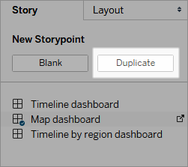
1. To use your first story point as a baseline for your next, click Duplicate under New Storypoint on the left.
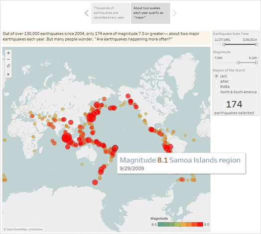
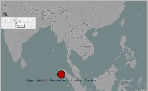
2. Change the Magnitude filter to 7.000 – 9.100 so that the map filters out smaller earthquakes. The map pans to show the Pacific “Ring of Fire (Link opens in a new window) ,” where the majority of the large earthquakes occurred.
3. Add a caption, such as About two quakes each year qualify as “major”
4. If you’re using Tableau Desktop, edit the description to describe what you’ve done in this story point. For example: Out of over 130,000 earthquakes since 2004, only 174 were of magnitude 7.0 or greater—about two major earthquakes each year. But many people wonder, “Are earthquakes happening more often?”
5. Click Update in the story toolbar above the caption to save your changes.

In the next story point, you’re going to drill down further, narrowing the story’s focus so that a specific type of earthquake—the “megaquake”—comes into view.

1. Click Duplicate in your second story point to use it as the baseline for your third story point.
2. Change the Magnitude filter to 8.000 – 9.100 so that the map filters out everything except the megaquakes.
3. Add the caption and description text.
   • Caption: These megaquakes have drawn a lot of attention
   • Description (Tableau Desktop only): Recent megaquakes of magnitude 8.0 and higher have often caused significant damage and loss of life. The undersea megaquakes near Indonesia and Japan also caused tsunamis that have killed many thousands of people.
4. Click Update to save your changes.

Highlight outliers

In the next two story points, you’re going to further engage your audience by examining data points at the far end of the scale: the two most deadly earthquakes in recent history.

1. As you’ve done before, use Duplicate to create a new story point as your starting point.
2. Adjust Magnitude to 9.000–9.100 and you’ll see just two data points.
3. Select one of the marks, such as the Indian Ocean earthquake and tsunami of 2004 that had a magnitude of 9.1.
4. Use the pan tool on the maps menu to center it in your story point.
5. Add caption and description text. For example:
   • Caption: The Indian Ocean earthquake and tsunami of 2004
   • Description (Tableau Desktop only): The 2004 Indian Ocean earthquake was an undersea megathrust earthquake that occurred on December 26, 2004. It is the third largest earthquake ever recorded and had the longest duration of faulting ever observed, between 8.3 and 10 minutes.
6. Click Update to save your changes.
7. Repeat the preceding steps for the Japanese earthquake and tsunami of 2011, using the following as caption and description text.
   • Caption: The Japanese earthquake and tsunami of 2011
   • Description (Tableau Desktop only): The 2011 quake off the coast of Tõhoku was a magnitude 9.0 undersea megathrust earthquake. It was the most powerful known earthquake ever to have hit Japan, and the 5th most powerful earthquake ever recorded.

Notice that you’ve already created a compelling visual story using just a single dashboard—all by filtering the data and zooming and panning the map.

We still haven’t answered the key question, however: Are big earthquakes on the rise? The next story points will dig in to that angle.

Show a trend

In the next story point, you’ll switch to a line chart (the Timeline dashboard) to show your audience a trend you spotted when you were initially creating views and dashboards.

1. Switch from the story you’re building to Timeline dashboard .
2. On the Timeline dashboard, set size to Fit to Earthquake story .
3. Go back to your story and click Blank to create a fresh story point.
4. Double-click the Timeline dashboard to add it to your story sheet. More earthquakes are being reported over time since 1973. In fact, it’s increased significantly!
5. Add a caption, such as: More and more earthquakes are being detected
6. Use Drag to add text to add a description of the trend (Tableau Desktop only): Since 1973, there’s been a steady increase in the number of earthquakes recorded. Since 2003, the trend has accelerated.

Offer your analysis

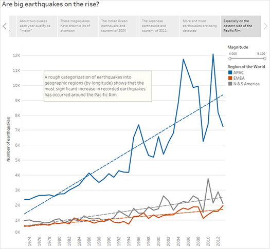
From your earlier work in this story with the Map dashboard you know that there are regional differences in earthquake frequency. In your next story point, you’ll pull in the Timeline by region dashboard , which breaks out earthquakes by region, and adds trend lines, which help reduce the variability in the data.

1. Click Blank to create a new story sheet.
2. Double-click the Timeline by region dashboard to the story sheet. The APAC region clearly stands out.
3. Add a caption then use Drag to add text to add a comment that points out the large number of earthquakes in the APAC region.
   • Caption: Especially on the eastern side of the Pacific Rim
   • Description (Tableau Desktop only): A rough categorization of earthquakes into geographic regions (by longitude) shows that the most significant increase in recorded earthquakes has occurred around the Pacific Rim.

Answer the question

Thus far, your data story has concluded that earthquake frequency in the Pacific Rim has increased since 1973, but your original question was about whether big earthquakes are becoming more frequent.

To answer this question, in your final story point, you’ll filter out weaker earthquakes and see what the resulting trend line is.

1. Click Duplicate to create a new story sheet.
2. Set the Magnitude filter to 5.000–9.100 . Notice how the trend lines have flattened out but there’s still a slight increase.
3. Add a caption then use Drag to add text to add your answer to the story point. Caption: But the trend in big quakes is not as clear Description (Tableau Desktop only): It appears that big earthquakes are increasing slightly. There should be more investigation, however, on whether this trend is real or the result of a small number of exceptionally strong recent earthquakes.As is often the case with a data story, the story ends with additional questions. Yes, there’s a trend, but it’s slight. More big earthquakes (magnitude 5.000 – 9.100) have been reported in recent years, especially in the Asia-Pacific region, but could that be natural variation? That might be a good topic for another story.

A short history

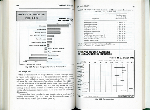
When Mary Eleanor Spear wrote her pioneering visualisation book Charting Statistics in 1952, she emphasised graphics that could be easily hand-drawn. For example, the ‘range bar chart’ (a predecessor of the boxplot) is a simple summary graphic for one numeric variable — a relatively simple visual to create without a computer.

Unlike a histogram, which would require deciding on breakpoints a priori and counting the number of cases that fall into each bin, a boxplot relies only on a few summary statistics. The analyst would calculate the median, the quartiles, and account for outliers, then get out their ruler and pencil to draw the visualisation.

John Tukey popularised these ideas in his 1977 book Exploratory Data Analysis, where he also emphasised that graphics could be easily hand-drawn.

The idea of Exploratory Data Analysis (now commonly abbreviated EDA) is to compute summary statistics and make basic data visualisations to understand a dataset before moving forward. Every graphic in the EDA book was made by hand by Tukey, although he was so precise they can be mistaken for computer-generated charts.

Jacques Bertin, another visualisation pioneer, was also focused on making a data analyst as effective as possible without a computer. One of his strategies was to create a ‘Bertin matrix’, a physical representation of an entire dataset, which could be reordered by the use of long skewers stuck through it. His graduate students would work to find an ordering that showed structure in the data, then photocopy the physical matrix to retain a version of the data before moving on.

Is digital better? A case for hand-drawing visuals

So, handmade data visualisation is not something new. In fact, it is the original form of visualisation! But, as computer tools have evolved to make it easier to create data visualisations, more and more visuals are ‘born digital’. That doesn’t mean the need for handmade visualisation has disappeared, or that computer-generated graphics are better. There are several reasons why I advocate for journalists to experiment with hand-drawing visuals:

1. It gets you thinking outside the box. If you are someone who is adept at using computer tools to generate visualisations, you may only think of the visual forms most easily generated by your tool.
2. A handmade visualisation can lend a feeling of friendliness to a story. Quite often, computer-generated visualisations feel sterile and can be inaccessible to certain audiences.
3. Handmade visualisations feel less ‘truthy’, so they can be a great way to convey uncertainty.
4. Making visualisations by hand is a concrete way to learn the way that data values are coupled to visual marks.
5. It’s fun!

Sometimes a handmade visualisation is a product you make for yourself, to help you brainstorm, understand your data, or just as a creative outlet. Other times, a handmade data visualisation can become your final product, published for others to read and experience.

And there are many handmade visualisations to draw inspiration from. The book Infographics Designers Sketchbooks is filled with behind-the-scenes looks at how visualisations began their lives. While some of the authors do their sketching in code, the vast majority begin by drawing on paper. So, hand-drawn visualisation can also be a step on the way to something computer-generated.

Perhaps more interesting are the hand-drawn visualisations that end up getting published in one way or another. In the category of personal visualisation, the project Dear Data, by Giorgia Lupi and Stefanie Posavec is a prime example.

The reports were works of art, like an autobiography in data visualisation.

Lupi and Posavec are both professional designers, and their client work (typically computer-generated) can be seen in a variety of contexts.

For Dear Data, they took another approach. Every week for a year, they each collected data on an agreed-upon topic about their lives (like laughter, doors, or complaints) and generated a hand-drawn visualisation of that data on a postcard. They mailed the postcards transatlantically to one another.

While data visualisations often aim to accurately convey information to a reader, that wasn’t the goal for Lupi and Posavec.

Instead, they wanted to convey some sense of their lives to one another. Readers aren’t asked to decipher the precise values they put on the page, but rather to draw inspiration from beautiful forms, and enjoy what is closer to a narrative or memoir of the authors’ lives.

There are other data artists who produce work in this space, like Nicholas Felton, who for years produced the annual ‘Feltron Report’.

People who bought the Feltron Report weren’t doing so in order to learn something new about the world, but to appreciate Felton’s work. Again, the reports were works of art, like an autobiography in data visualisation.

What the experts say

Research on data visualisation often focuses on how effective a visualisation is at conveying the precise information it encodes. In 1984, William Cleveland and Robert McGill published a paper called Graphical perception: Theory, experimentation, and application to the development of graphical methods.

This paper (cited more than 1,600 times!) outlined the results of their experiments on graphical perception. If you have heard arguments for the use of bar charts instead of pie charts, the data likely came from this 1984 study.

Their study showed how bad people are at judging areas (of circles or other shapes) and cautioned against the use of area as a method for graphical encoding. IEEE Vis, a professional community and conference for computer scientists studying visualisation, continues to publish papers along these lines.

For example, the paper Ranking Visualizations of Correlation Using Weber’s Law, demonstrated which data visualisations made it easiest for readers to assess correlation visually.

However, the goal of visualisation does not always have to be to encode information in such a way that it is easy to read off exact values. Often, the most important thing is to give a truthful impression of the data. And, the most technically correct visualisations may not always be the best way to convey that impression.

Often, the most important thing is to give a truthful impression of the data.

One important component of visualisation is attention — a person can’t read and understand a visual unless they pay attention to it. Visualisation critic Edward Tufte often advocates for the simplest possible visualisation, by maximising the data-ink ratio.

Darkhorse Analytics produced a gif example of what this process could look like. In many cases, it is better to reduce the amount of visual clutter and non-data ink, but other times it seems Tufte takes this too far, such as his redesign of the boxplot that ends up as a broken line with a dot in the centre.

Data visualisation expert Nathan Yau advocates for what he calls ‘whizbang’. Whizbang is the cool factor (often animation or interaction) that draws people into your visualisations. In a world filled with digitally-generated visualisations, a handmade visualisation might be just the whizbang you need to draw readers in.

Data journalist Mona Chalabi has embraced this idea, creating many hand-drawn visualisations that are published as finished pieces in The Guardian and elsewhere.

Chalabi is the data editor at The Guardian, so she knows the ‘rules’ of data visualisation. But she also understands when it makes sense to bend or break them. Her OpenVisConf talk, Informing without Alienating, discusses her philosophy of making graphics that inform as many people as possible.

Chalabi considers the context in which her visualisations will be seen. She also draws her visualisations using familiar objects, to help readers understand things like units. For example, she created a visualisation to answer the question ’How much pee is a lot of pee?’ using common soda bottle sizes:

View this post on Instagram

In another piece, she showed sugar consumption over time in the US and the UK, using sugar sprinkles.

View this post on Instagram

Beyond the familiarity granted by the objects Chalabi draws, the hand-drawn nature of her visualisations make them feel less precise. Again, this is her intention. Numbers and computer-generated visualisations often ‘feel’ true, but there is always some amount of uncertainty that surrounds them.

By drawing her visualisations, Chalabi is able to convey some amount of variability. When you look at her visualisation of how much air pollution is emitted and inhaled by people of different races, you won’t be able to read off the exact numbers. (In fact, you can’t read off numbers at all — the chart does not have labeled axes!) Instead, you will be able to see which group’s share is largest, and by how much.

View this post on Instagram

Chalabi is working from her gut, but researchers at Bucknell University have begun to study how different groups interpret data visualisations differently. So far they have focused on a particular rural population, but you can imagine how this work could be extended to other subgroups. One of their key findings is that visualisations are personal.

Often, we imagine that we can generate an idealised representation of a particular dataset, but everyone comes to our visualisations with their own identity and prior beliefs. For certain groups, a visualisation may work well, and for others not at all.

Bucknell’s researchers point out that many of the field’s historic studies on perception relied upon a homogeneous group of people (often, college students, who tend to be whiter, richer, and, of course, more educated than the general population).